CONVOLUTION

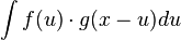
In mathematics and, in particular, functional analysis, convolution is a mathematical operation on two functions f and g, producing a third function that is typically viewed as a modified version of one of the original functions, giving the area overlap between the two functions as a function of the amount that one of the original functions is translated. Convolution is similar tocross-correlation. It has applications that include probability, statistics, computer vision, natural language processing, imageand signal processing, engineering, and differential equations.

The convolution can be defined for functions on groups other than Euclidean space. For example, periodic functions, such as the discrete-time Fourier transform, can be defined on a circle and convolved by periodic convolution. (See row 10 atDTFT#Properties.)  And discrete convolution can be defined for functions on the set of integers. Generalizations of convolution have applications in the field of numerical analysis and numerical linear algebra, and in the design and implementation of finite impulse response filters in signal processing.

Computing the inverse of the convolution operation is known as deconvolution.

                               

Historical developments

One of the earliest uses of the convolution integral appeared in D'Alembert's derivation of Taylor's theorem in Recherches sur différents points importants du système du monde,published in 1754.^[1]

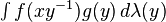
Also, an expression of the type:

is used by Sylvestre François Lacroix on page 505 of his book entitled Treatise on differences and series, which is the last of 3 volumes of the encyclopedic series: Traité du calcul différentiel et du calcul intégral, Chez Courcier, Paris, 1797-1800.^[2] Soon thereafter, convolution operations appear in the works of Pierre Simon Laplace, Jean Baptiste Joseph Fourier, Siméon Denis Poisson, and others. The term itself did not come into wide use until the 1950s or 60s. Prior to that it was sometimes known as faltung (which means folding in German), composition product, superposition integral, and Carson's integral.^[3] Yet it appears as early as 1903, though the definition is rather unfamiliar in older uses.^[4][5]

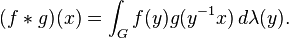
The operation:

Fast convolution algorithms

In many situations, discrete convolutions can be converted to circular convolutions so that fast transforms with a convolution property can be used to implement the computation. For example, convolution of digit sequences is the kernel operation in multiplication of multi-digit numbers, which can therefore be efficiently implemented with transform techniques (Knuth 1997, §4.3.3.C; von zur Gathen & Gerhard 2003, §8.2).

Eq.1 requires N arithmetic operations per output value and N² operations for N outputs. That can be significantly reduced with any of several fast algorithms. Digital signal processing and other applications typically use fast convolution algorithms to reduce the cost of the convolution to O(N log N) complexity.

The most common fast convolution algorithms use fast Fourier transform (FFT) algorithms via the circular convolution theorem. Specifically, the circular convolution of two finite-length sequences is found by taking an FFT of each sequence, multiplying pointwise, and then performing an inverse FFT. Convolutions of the type defined above are then efficiently implemented using that technique in conjunction with zero-extension and/or discarding portions of the output. Other fast convolution algorithms, such as theSchönhage–Strassen algorithm or the Mersenne transform,^[9] use fast Fourier transforms in other rings.

If one sequence is much longer than the other, zero-extension of the shorter sequence and fast circular convolution is not the most computationally efficient method available.^[10]Instead, decomposing the longer sequence into blocks and convolving each block allows for faster algorithms such as the Overlap–save method and Overlap–add method.^[11] A hybrid convolution method that combines block and FIR algorithms allows for a zero input-output latency that is useful for real-time convolution computations

If G is a suitable group endowed with a measure λ, and if f and g are real or complex valued integrable functions on G, then we can define their convolution by

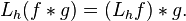
It is not commutative in general. In typical cases of interest G is a locally compact Hausdorff topological group and λ is a (left-) Haar measure. In that case, unless G isunimodular, the convolution defined in this way is not the same as . The preference of one over the other is made so that convolution with a fixed function g commutes with left translation in the group:

Furthermore, the convention is also required for consistency with the definition of the convolution of measures given below. However, with a right instead of a left Haar measure, the latter integral is preferred over the former.

On locally compact abelian groups, a version of the convolution theorem holds: the Fourier transform of a convolution is the pointwise product of the Fourier transforms. Thecircle group T with the Lebesgue measure is an immediate example. For a fixed g in L¹(T), we have the following familiar operator acting on the Hilbert space L²(T):

The operator T is compact. A direct calculation shows that its adjoint T* is convolution with

By the commutativity property cited above, T is normal: T*T = TT*. Also, T commutes with the translation operators. Consider the family S of operators consisting of all such convolutions and the translation operators. Then S is a commuting family of normal operators. According to spectral theory, there exists an orthonormal basis {h_k} that simultaneously diagonalizes S. This characterizes convolutions on the circle. Specifically, we have

which are precisely the characters of T. Each convolution is a compact multiplication operator in this basis. This can be viewed as a version of the convolution theorem discussed above.

A discrete example is a finite cyclic group of order n. Convolution operators are here represented by circulant matrices, and can be diagonalized by the discrete Fourier transform.

A similar result holds for compact groups (not necessarily abelian): the matrix coefficients of finite-dimensional unitary representations form an orthonormal basis in L² by thePeter–Weyl theorem, and an analog of the convolution theorem continues to hold, along with many other aspects of harmonic analysis that depend on the Fourier transform.

Convolution of measures

Let G be a topological group. If μ and ν are finite Borel measures on G, then their convolution μ∗ν is defined by

for each measurable subset E of G. The convolution is also a finite measure, whose total variation satisfies

In the case when G is locally compact with (left-)Haar measure λ, and μ and ν are absolutely continuous with respect to a λ, so that each has a density function, then the convolution μ∗ν is also absolutely continuous, and its density function is just the convolution of the two separate density functions.

If μ and ν are probability measures on the topological group (R,+), then the convolution μ∗ν is the probability distribution of the sum X + Y of two independent random variables Xand Y whose respective distributions are μ and ν.

Applications

Gaussian blur can be used in order to obtain a smooth grayscale digital image of a halftone print

Convolution and related operations are found in many applications in science, engineering and mathematics.

• In image processing

See also: digital signal processing

In digital image processing convolutional filtering plays an important role in many important algorithms in edge detection and related processes.

In optics, an out-of-focus photograph is a convolution of the sharp image with a lens function. The photographic term for this isbokeh.

In image processing applications such as adding blurring.

• In digital data processing

In analytical chemistry, Savitzky–Golay smoothing filters are used for the analysis of spectroscopic data. They can improve signal-to-noise ratio with minimal distortion of the spectra.

In statistics, a weighted moving average is a convolution.

• In acoustics, reverberation is the convolution of the original sound with echoes from objects surrounding the sound source.

In digital signal processing, convolution is used to map the impulse response of a real room on a digital audio signal.

In electronic music convolution is the imposition of a spectral or rhythmic structure on a sound. Often this envelope or structure is taken from another sound. The convolution of two signals is the filtering of one through the other.^[15]

• In electrical engineering, the convolution of one function (the input signal) with a second function (the impulse response) gives the output of a linear time-invariant system (LTI). At any given moment, the output is an accumulated effect of all the prior values of the input function, with the most recent values typically having the most influence (expressed as a multiplicative factor). The impulse response function provides that factor as a function of the elapsed time since each input value occurred.
• In physics, wherever there is a linear system with a "superposition principle", a convolution operation makes an appearance. For instance, in spectroscopy line broadening due to the Doppler effect on its own gives a Gaussian spectral line shape and collision broadening alone gives a Lorentzian line shape. When both effects are operative, the line shape is a convolution of Gaussian and Lorentzian, a Voigt function.

In Time-resolved fluorescence spectroscopy, the excitation signal can be treated as a chain of delta pulses, and the measured fluorescence is a sum of exponential decays from each delta pulse.

In computational fluid dynamics, the large eddy simulation (LES) turbulence model uses the convolution operation to lower the range of length scales necessary in computation thereby reducing computational cost.

• In probability theory, the probability distribution of the sum of two independent random variables is the convolution of their individual distributions.

In kernel density estimation, a distribution is estimated from sample points by convolution with a kernel, such as an isotropic Gaussian. (Diggle 1995).

• In radiotherapy treatment planning systems, most part of all modern codes of calculation applies a convolution-superposition algorithm